Compressing Earth Embeddings
Update (2026-03-26): OlmoEarth-nano results throughout have been recomputed with properly normalized inputs. The initial version we released used unnormalized inputs, which significantly underestimated OlmoEarth-nano’s performance. Thanks Gabriel Tseng for flagging this issue!
Foundation models like Tessera [1], OlmoEarth [2], and AlphaEarth [3] produce dense per-pixel embeddings from satellite imagery. With a kNN classifier or linear probe, you can do classification, change detection, or similarity search — no fine-tuning needed. The appeal here is that you can skip expensive image preprocessing and model inference, download some embeddings, then plug into your task. But the cost of actually storing these embedding products can get out of hand fast.
Isaac’s recent survey of earth embedding products [4] catalogued this growing ecosystem — AlphaEarth, Tessera, Clay, Major-TOM, MOSAIKS — and identified a common problem: at continental or global scale, embedding storage costs dwarf the compute savings that motivated precomputation in the first place. Distribution is fragmented across incompatible formats (COG, GeoParquet, raw NumPy), and there are no shared standards for tiling, CRS, or provenance. But the most fundamental issue is size.
The storage problem
Earth’s land surface covers about 150 million km^2. At Sentinel-2’s 10m resolution, that’s 1.5 trillion pixels. Multiply by embedding dimension and bytes per element:
| Model | Dims | Bytes/embedding | 1 year (global) | S3 cost/year |
|---|---|---|---|---|
| DINOv3 ViT-L (float32) | 1,024 | 4,096 | 6.1 PB | $1.7M |
| DINOv3 ViT-L (int8) | 1,024 | 1,024 | 1.5 PB | $424K |
| Tessera encoder (float32) | 512 | 2,048 | 3.1 PB | $847K |
| Tessera product (int8) | 128 | 128 | 192 TB | $53K |
| OlmoEarth-nano (float32) | 128 | 512 | 768 TB | $212K |
| AEF (int8) | 64 | 64 | 96 TB | $26K |
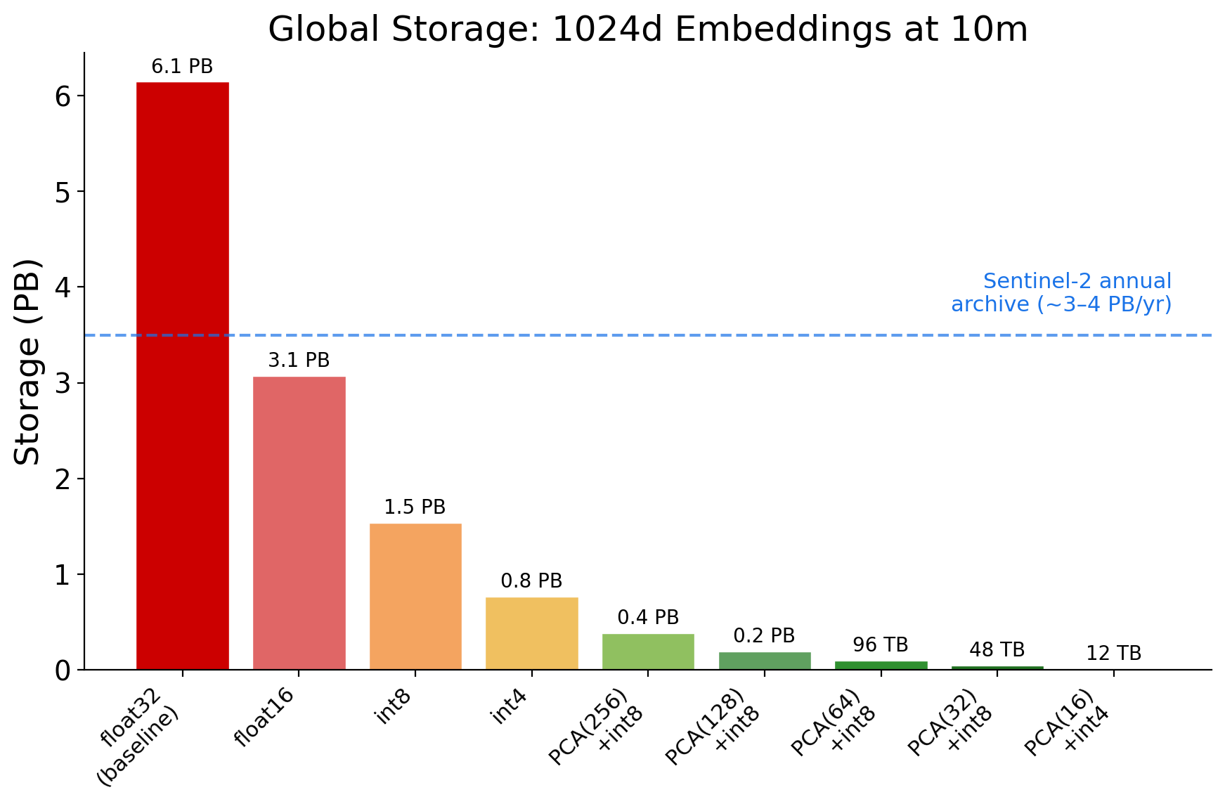
For context, the entire Sentinel-2 archive — every L1C and L2A product collected since 2015 — was roughly 22 PB in 2022 [5] and exceeded 50 PB by mid-2025 [6]. The archive grows by 3-4 PB per year. A single year of 1024d float32 embeddings (6.1 PB) would exceed the annual Sentinel-2 data volume that produced them. The embeddings are larger than the source imagery.
The embeddings are larger than the source imagery.
And these are per-year numbers. AlphaEarth covers 2017-2025 (9 years). Tessera plans the same. Multi-year archives at these scales reach tens of petabytes even for compact models. So how much can you compress before the embeddings stop being useful?
EO representations are redundant
Two recent papers provide evidence that earth observation representations carry substantial redundancy.
Model-level redundancy. Hackel et al. [7] applied post-hoc “slimming” to remote sensing foundation models — uniformly reducing the width of transformer layers after training. At just 1% of the original FLOPs, these models retained over 71% of their full-scale accuracy (relative retention). An ImageNet-trained MAE dropped below 10% relative retention under the same treatment. Intermediate model sizes sometimes outperformed the full model, suggesting the extra capacity adds noise rather than signal. If the intermediate representations are this redundant, the output embeddings are too.
Image-level redundancy. Papazafeiropoulos et al. [8] applied patch-level masking during training and inference of a ViT model, retaining only a fraction of image patches. On BigEarthNet, 15% patch retention achieved 99.4% of baseline accuracy. Even segmentation tolerated 50% patch removal while recovering ~97% of full performance.
These results suggest that standard embedding compression methods — including quantization and dimensionality reduction — may be effective for remotely sensed data as well. So we tested it!
Experimental setup
We evaluate combinations of quantization (float32, int8, int4, int2, binary, ternary, product quantization) and dimensionality reduction (PCA, truncated SVD, random projection, feature selection) across 5 embedding models and 6 classification datasets.
All experiments in this section use EuroSAT [9] — a 10-class Sentinel-2 land cover dataset with 21,600 images — as the primary benchmark. We use the precomputed embeddings for AEF, OlmoEarth, and Tessera from Isaac’s geopool repository, and we compute DINOv3 and ResNet50 embeddings separately. Then, we validate our findings on 5 additional datasets (RESISC45 [10] and 4 GeoBench [11] benchmarks) with the DINOv3 and ResNet50 based embeddings in the cross-dataset section below.
Models
| Model | Architecture | Dims | Bytes/emb | Pretraining |
|---|---|---|---|---|
| AlphaEarth (AEF) | STP Encoder | 64 | 256 | 3B+ multi-source EO obs. |
| OlmoEarth-nano | Transformer | 128 | 512 | S1/S2/Landsat self-supervised |
| Tessera | Transformer | 512 | 2,048 | S1/S2 self-supervised |
| DINOv3 ViT-L/16 | Vision Transformer | 1,024 | 4,096 | SAT-493M (0.6m Maxar RGB) |
| ResNet50 | CNN | 2,048 | 8,192 | ImageNet supervised |
DINOv3 ViT-L/16 uses Meta’s SAT-493M checkpoint [12] — a ViT-L distilled from the DINOv3 ViT-7B, trained on 493 million 0.6m Maxar RGB tiles. Tessera’s encoder outputs 512-dim embeddings, but the distributed product compresses these to 128-dim int8 with per-pixel scale factors. Our experiments use the 512-dim encoder output via geopool.
We evaluate with kNN (k=5, cosine distance) and linear probes (logistic regression with tuned regularization). All quantization and reduction parameters are fit on training data only. DINOv3 results use mean-pooled patch tokens throughout unless noted.
Baselines
| Model | Dims | B/emb | EuroSAT kNN | EuroSAT Linear |
|---|---|---|---|---|
| AEF | 64 | 256 | 94.5% | 95.4% |
| OlmoEarth-nano | 128 | 512 | 94.8% | 96.5% |
| Tessera | 512 | 2,048 | 87.6% | 94.2% |
| DINOv3 | 1,024 | 4,096 | 94.5% | 98.0% |
| ResNet50 | 2,048 | 8,192 | 92.6% | 95.8% |
int8 is always free
The simplest compression: reduce each float32 value to int8. For each dimension, compute the min and max across the training set, then linearly map the range into 256 integer levels (4x compression).
| Method | Bits | B/emb (1024d) | AEF | OlmoEarth-nano | Tessera | DINOv3 | ResNet50 |
|---|---|---|---|---|---|---|---|
| float32 | 32 | 4,096 | 94.5% | 94.8% | 87.6% | 94.5% | 92.6% |
| int8 | 8 | 1,024 | 94.6% | 94.8% | 87.8% | 94.5% | 92.5% |
| int4 | 4 | 512 | 94.2% | 94.4% | 86.5% | 94.4% | 92.4% |
| int2 | 2 | 256 | 91.7% | 91.0% | 84.7% | 92.3% | — |
| binary | 1 | 128 | 88.8% | 90.8% | 81.4% | 91.8% | 86.8% |
EuroSAT kNN accuracy. Bold row = statistically indistinguishable from float32 baseline.
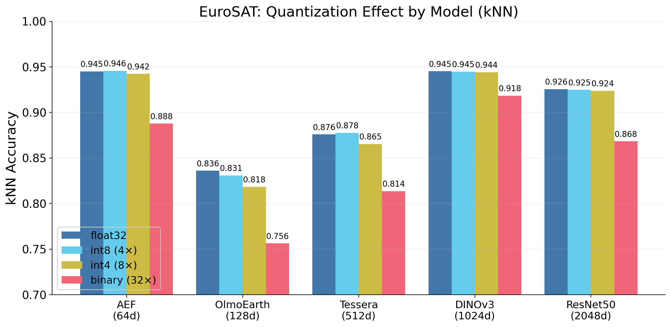
We find int8 is never statistically distinguishable from float32. McNemar’s test gives p >= 0.12 for every model-dataset pair (smallest p = 0.12). The 95% bootstrap confidence interval for the accuracy difference is within +/-0.2% everywhere. There is no reason to store float32 embeddings.
There is no reason to store float32 embeddings.
We also find int4 loses less than 1% for AEF and DINOv3. Binary quantization (1 bit per dimension, 32x compression) is worth a closer look — DINOv3 at 128 bytes still hits 91.8%! More on this below.
Most embedding dimensions are redundant
PCA variance analysis reveals different spectral structures across models:
| Model | 4d | 8d | 16d | 32d | 64d | 256d |
|---|---|---|---|---|---|---|
| AEF (64d) | 57% | 80% | 91% | 97% | 100% | — |
| OlmoEarth-nano (128d) | 77% | 88% | 95% | 98% | 100% | — |
| Tessera (512d) | 94% | 98% | 99% | 100% | 100% | 100% |
| DINOv3 mean (1024d) | 52% | 64% | 74% | 82% | 88% | 97% |
| DINOv3 cls (1024d) | 35% | 46% | 57% | 67% | 76% | 91% |
Cumulative variance explained by top-k PCA components, fitted on EuroSAT training embeddings.
OlmoEarth-nano spreads its variance more broadly than Tessera, with 77% in 4 dimensions and needing 32 dimensions for 98%. DINOv3 distributes variance more evenly still, needing 256 dimensions for 97%.
DINOv3 spreads its variance across many dimensions, so you might expect it to compress poorly — if no dimension is dispensable, PCA can’t help. But DINOv3 at PCA(64)+int8 (6% of its original dimensions) still hits 93.1% kNN accuracy, only 1.4% below baseline. The dimensions PCA discards carry variance but apparently not much task-relevant information.
Combined compression: the Pareto frontier
The best configurations combine PCA with quantization — reduce dimensions first, then quantize:
| Model | Config | B/emb | EuroSAT kNN | EuroSAT Linear |
|---|---|---|---|---|
| AEF | int8 | 64 | 94.6% | 95.5% |
| AEF | int4 | 32 | 94.2% | 95.0% |
| DINOv3 | int8 | 1,024 | 94.5% | 98.0% |
| DINOv3 | int4 | 512 | 94.4% | 97.9% |
| DINOv3 | PCA(128)+int8 | 128 | 93.6% | 97.3% |
| DINOv3 | PCA(64)+int8 | 64 | 93.1% | 96.4% |
| DINOv3 | PCA(32)+int8 | 32 | 92.4% | 94.1% |
| DINOv3 | PCA(16)+int4 | 8 | 89.3% | 90.5% |
EuroSAT accuracy. kNN: k=5, cosine. Linear: logistic regression, C tuned.
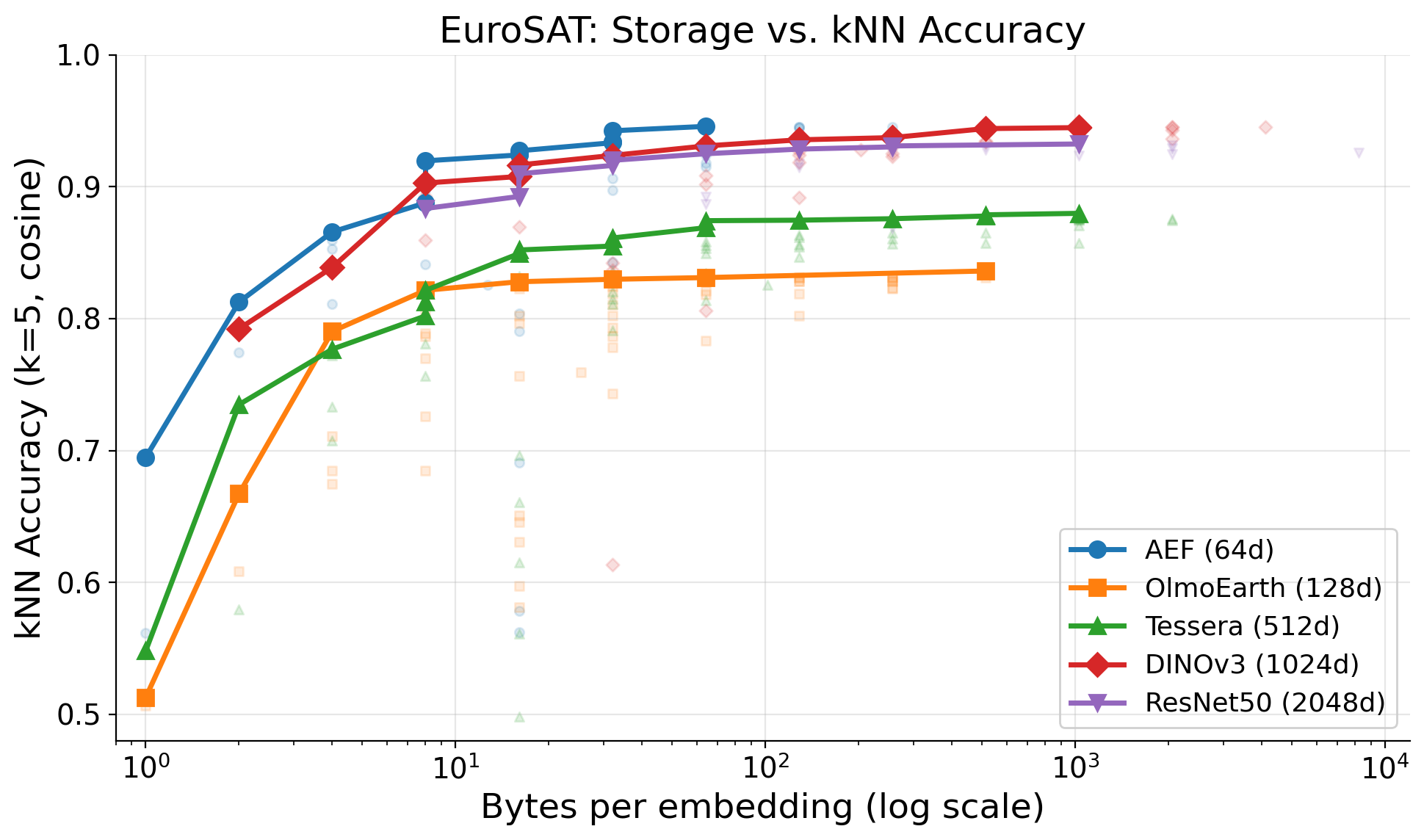
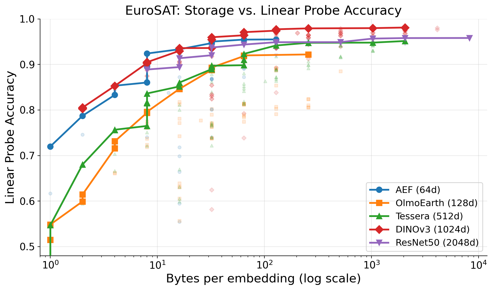
The two plots tell different stories. For kNN, AEF dominates at every storage budget — its 64 dimensions are compact enough that int8 at 64 bytes is nearly unbeatable, and larger models can’t overcome the dimensionality tax. For linear probes, DINOv3 pulls ahead once budgets exceed ~16 bytes, because a trained classifier can exploit the richer representation even after PCA compression.
PCA(64)+int8 at 64 bytes/embedding is the sweet spot for DINOv3: 64x compression with only 1.4% kNN loss and 96.4% linear accuracy. That brings a year of global DINOv3 embeddings from 6.1 PB down to 96 TB — the same footprint as AlphaEarth’s native int8 representation. Which model to choose depends on your task: kNN retrieval favors AEF, classification with a trained head favors DINOv3.
Binary quantization on DINOv3
DINOv3 loses only 2.7% kNN accuracy under binary quantization (1 bit per dimension, 32x compression), while AEF and Tessera lose 5.7-6.2%. We hypothesize that this might be due to:
High dimensionality. 1,024 binary dimensions give 2^1024 possible codes — enormous capacity for separating 10 classes.
Balanced dimensions. DINOv3’s dimensions are nearly symmetric around their means (average imbalance = 0.018). Each threshold bit carries close to 1 bit of entropy. OlmoEarth-nano is also well-balanced (0.052), while AEF’s higher imbalance (0.082) means many bits are nearly constant.
A related finding with the binary quantizations: Hamming distance on raw bits outperforms reconstructing float32 vectors and computing cosine distance. The reconstruction step replaces each bit with a centroid value (the mean of all above-threshold or below-threshold values for that dimension). We find that KNN with a Hamming distance (count the differing bits between the two vectors) outperforms using cosine distance on the reconstructed vectors. This seems to preserve the ranking of neighbor distances better:
| Model | Dims | Baseline | Reconstructed + cosine | Hamming on raw bits |
|---|---|---|---|---|
| DINOv3 | 1,024 | 94.5% | 91.8% | 93.2% |
| Tessera | 512 | 87.6% | 81.4% | 87.0% |
| OlmoEarth-nano | 128 | 94.8% | 90.8% | 92.7% |
| AEF | 64 | 94.5% | 88.8% | 89.1% |
Hamming distance is also significantly faster to compute than cosine distance on reconstructed vectors — it reduces to a popcount on XOR’d bit vectors.
Cross-dataset consistency
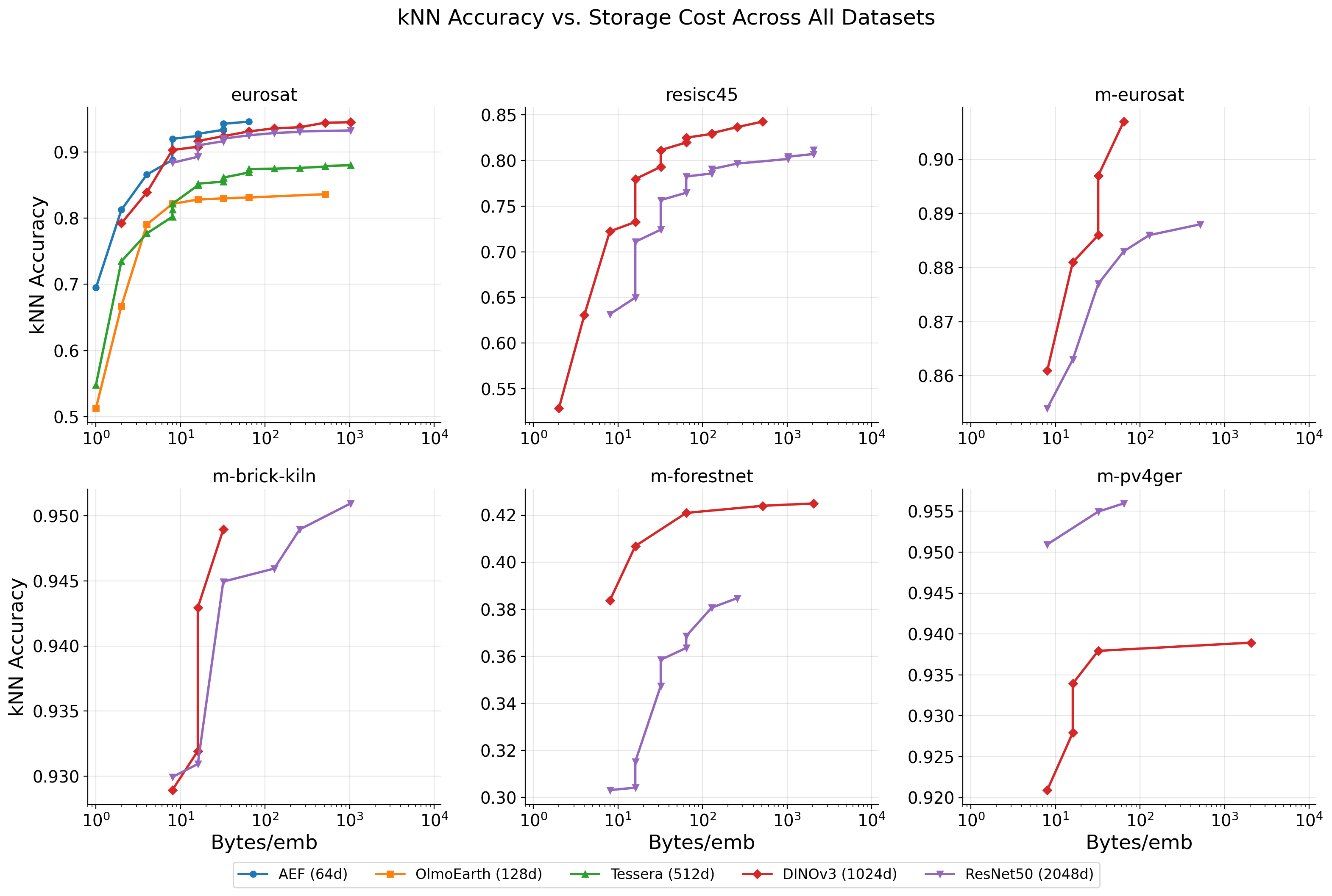
The compression patterns hold across all 6 datasets:
- int8 is effectively lossless on all datasets, including the 45-class RESISC45.
- PCA(64)+int8 at 64 bytes gives 93.1% on EuroSAT (10 classes) and 82.0% on RESISC45 (45 classes) — proportionally similar retention.
- m-forestnet (deforestation driver classification) is the hardest task at ~40% kNN for DINOv3 and ~36% for ResNet50 — likely because RGB-only embeddings lose the spectral bands needed for this task.
Per-class failure modes
Under aggressive compression, specific classes are disproportionately affected:
| Model | Config (B/emb) | Worst class | F1 drop |
|---|---|---|---|
| AEF | int4 (32 B) | Highway | -0.012 |
| AEF | binary (8 B) | Highway | -0.170 |
| AEF | PCA(8)+binary (1 B) | Highway | -0.486 |
| OlmoEarth-nano | PCA(8)+binary (1 B) | PermanentCrop | -0.570 |
| Tessera | PCA(8)+binary (1 B) | PermanentCrop | -0.479 |
Highway and PermanentCrop are consistently the most affected — narrow categories relying on fine-grained spectral or spatial features that aggressive quantization destroys. If your application needs balanced per-class performance (rare category detection, e.g.), avoid extreme compression and verify per-class metrics.
Limitations
The main experiments here use EuroSAT — a 10-class patch classification dataset that most models find relatively easy (baselines already at 94-98%). We have some evidence from DINOv3 and ResNet50 results on RESISC45 (45 classes) and 4 GeoBench benchmarks that the core findings generalize across patch classification tasks — int8 is effectively lossless on all of them. But all 6 datasets are patch classification. We have not tested:
- Semantic segmentation — pixel-level predictions may be more sensitive to per-dimension quantization error
- Pixel regression (e.g., canopy height, biomass estimation) — continuous targets could amplify small reconstruction errors that classification absorbs
- Object detection — localization accuracy may degrade differently than classification accuracy
- Change detection — differencing compressed embeddings across time steps could compound quantization noise
- Retrieval — ranking quality over large databases may be more sensitive to distance distortion than top-1 classification
If you are saving embeddings for one of these tasks, we recommend validating compression effects on a representative sample before committing to a storage format.
We also only test OlmoEarth-nano (1.4M params, 128d) — the smallest model in the OlmoEarth family. The larger variants (Tiny at 192d, Base at 768d, Large at 1024d) may have different compression characteristics. And input normalization and patch size play a role in downstream performance that we haven’t disentangled from the compression effects here.
Takeaways
Some takeaways from these experiments (given the above caveat about patch classification):
Always use int8. It is statistically indistinguishable from float32 across every model and dataset we tested (p > 0.12). 4x compression, zero engineering effort, no reason not to.
Check intrinsic dimensionality before storing. Many geospatial embeddings carry redundant dimensions. Tessera packs 94% of its variance into 4 dimensions; even DINOv3 can be PCA-reduced to 64d with only 1.5% kNN loss.
PCA(64)+int8 is the sweet spot for DINOv3. 64 bytes/embedding, 64x compression, 1.4% kNN loss, 96.4% linear accuracy.
For binary search indices, use Hamming distance directly on binary embeddings. Skip dequantization — it introduces correlated noise that hurts more than it helps.
Don’t use ternary quantization. Binary is simpler, uses fewer bits, and performs better in every configuration we tested.
Tune regularization (C) for linear probes. The default C=1.0 leaves performance on the table: Tessera gains 0.9% from C=10, DINOv3 gains 0.4% from C=0.1.
Verify per-class metrics under compression. Highway and PermanentCrop degrade disproportionately — aggregate accuracy can mask category-level failures.
Bibliography
[1] Feng, Z., et al. “Tessera: Global-Scale Pixel Embeddings from Sentinel-2.” arXiv:2506.20380, 2025. [paper] [code]
[2] Herzog, H., et al. “OlmoEarth: Stable Latent Image Modeling for Multimodal Earth Observation.” arXiv:2511.13655, 2025. [paper] [code]
[3] Brown, C.F., et al. “AlphaEarth Foundations: An embedding field model for accurate and efficient global mapping from sparse label data.” arXiv:2507.22291, 2025. [paper] [GEE catalog]
[4] Fang, H., et al. “Earth Embeddings as Products.” arXiv:2601.13134, 2026. [paper] [blog]
[5] Bauer-Marschallinger, B. and Falkner, K. “Wasting Petabytes: A Survey of the Sentinel-2 UTM Tiling Grid and its Spatial Overhead.” ISPRS Journal of Photogrammetry and Remote Sensing, 2023. [paper]
[6] ESA. “Copernicus Sentinels Mission and Data Management.” Living Planet Symposium, 2025. [slides]
[7] Hackel, L., Burgert, T., and Demir, B. “How Much of a Model Do We Need? Redundancy and Slimmability in Remote Sensing Foundation Models.” arXiv:2601.22841, 2026. [paper]
[8] Papazafeiropoulos, T., et al. “Hide and Seek: Investigating Redundancy in Earth Observation Imagery.” arXiv:2603.13524, 2026. [paper]
[9] Helber, P., et al. “EuroSAT: A Novel Dataset and Deep Learning Benchmark for Land Use and Land Cover Classification.” IEEE JSTARS, 2019. [paper]
[10] Cheng, G., Han, J., and Lu, X. “Remote Sensing Image Scene Classification: Benchmark and State of the Art.” Proceedings of the IEEE, 2017. [paper]
[11] Lacoste, A., et al. “GEO-Bench: Toward Foundation Models for Earth Monitoring.” NeurIPS, 2023. [paper]
[12] Simeoni, O., et al. “DINOv3” arXiv:2508.10104, 2025. [paper] [code]
Citation
@online{robinson2026,
  author = {Robinson, Caleb and Corley, Isaac},
  title = {Compressing {Earth} {Embeddings}},
  date = {2026-03-24},
  url = {https://geospatialml.com/posts/compressing-earth-embeddings/},
  langid = {en}
}