Gaussian Splat-based Satellite Image Super Resolution
Super-resolution is the task of recovering a higher-resolution image from one or more lower-resolution observations of the same scene. In the commercial satellite world, it’s now a product as companies aim to create sharper, more detailed imagery from their data. Planet’s recently released SuperRes product sharpens ~3m PlanetScope imagery to 2m, DigiFarm’s DR imagery takes 10m Sentinel-2 to 1m, and Vantor’s HD imagery takes 30cm to 15cm.
Academic work on the same problem goes back decades. Classical multi-frame super-resolution [1] showed that many shifted low-resolution observations of the same scene can be fused into a sharper image given a known imaging model and the inter-frame shifts. Sentinel-2-specific work has mostly taken a learned route since: Razzak et al. [2] fuse multi-temporal and multi-spectral cues with radiometric-consistency losses, and Aybar et al. [3] introduce SEN2SR, a deep-learning framework that pushes Sentinel-2 to 2.5m, benchmarks CNN, Mamba, and Swin Transformer backbones, and adds a low-frequency hard constraint to preserve spectral consistency. Sirko et al. [4] sidestep image super-resolution as an intermediate product, instead training an impressive Sentinel-2 student model to mimic 50 cm building and road predictions from a high-resolution teacher.
Super-resolution is also useful outside remote sensing. NVIDIA’s DLSS renders games at a lower internal resolution and learns to upscale. The trick DLSS exploits is that real scenes have structure, so a representation that captures that structure carries more detail per parameter than a dense pixel grid. In 3D vision, the dominant version is the Gaussian splat, a scene represented as anisotropic Gaussians over a continuous domain, fit by optimization rather than trained. Splats are continuous, have a closed-form forward model, and act as a smoothness prior that denoises without hallucinating detail. Pix4D’s photogrammetry pipeline and ArcGIS Reality both use splats to reconstruct sharp 3D scenes from photogrammetric imagery.
In this post we try using these recent ideas from the Gaussian splatting world to superresolve Sentinel-2 imagery timeseries.
Super resolving with Sentinel-2
The Sentinel-2 constellation revisits every spot on Earth roughly every 5 days. Over a single cloud-free summer at a mid-latitude site, that’s around 30 looks at the same patch of ground from the same sensor family. Although the delivered L2A products live on a fixed 10m UTM grid, the scene content is not perfectly co-registered across dates. Residual processing and viewing-geometry effects show up as sub-pixel translations between products: typically around 1.5m of standard deviation per axis, and occasionally as much as 6 to 7m. That small difference is what classical multi-frame super-resolution exploits. Given many slightly shifted samples of the same scene, you can solve for the hidden high-resolution image that, once shifted, blurred, and downsampled the way the sensor would, reproduces every observation.
To do this, we represent the ground as a continuous field of 2D Gaussian splats on a fine grid, push it through an analytic forward model, and let a gradient based optimizer (LBFGS) jointly recover the scene weights and per-observation shifts. The implementation is around 500 lines of PyTorch, and the optimizer rediscovers the sub-pixel jitter on its own.
Background: the point-spread function
Every camera and sensor blurs a single point of light into a small fuzzy spot. That spot is the point-spread function, or PSF. It comes from the optics, the atmosphere, and the sensor’s photodetector response.
For a satellite imager, the PSF is typically wider than a single pixel on the ground. The optics smear features smaller than the PSF across several pixels before the sensor digitizes anything, so post-processing alone cannot put that information back without an external prior.
The cleanest analogy is a long-exposure photo of an out-of-focus star: stacking more exposures averages down the noise, but never recovers what’s inside the blurred disk.
For Sentinel-2’s 10m bands, the residual blur after pixel aperture is approximately a 2D Gaussian with a standard deviation of roughly 3 to 5m.1 Without an external or learned prior, you should not expect to reliably recover arbitrary features much below roughly the 8–10 m scale from Sentinel-2.
Our forward model includes the PSF as an explicit known-Gaussian blur. The assumed PSF width matters more than any other knob. Too narrow and the model invents detail that isn’t there. Too wide and it can’t resolve anything.
The setup
We pull 32 cloud-free L2A scenes from April–October 2025 over a 987 × 1011 pixel area at 10m resolution from the Microsoft Planetary Computer. Most ablations and visual examples below use a centred 256 × 256 pixel crop (2.56 × 2.56 km) of that scene. We co-register four bands (B02, B03, B04, B08, corresponding to Blue, Green, Red, and NIR) into a single time series. Esri World Imagery (~0.8m/px) over the same AOI is used only as a visual reference.
The model treats all observations as views of one latent scene. That only works when temporal variation (phenology, illumination, atmosphere, BRDF) is small relative to the spatial structure we care about. A tighter seasonal window or per-date radiometric correction would help on dynamic landscapes.
The job is an inverse problem: we never see the high-resolution scene \(x\) directly; we see 32 low-resolution measurements \(\{y_t\}\). The forward model that maps the hidden scene to each measurement is
\[ y_t \;=\; D \cdot H \cdot W_t(x) \;+\; \varepsilon_t, \]
where \(W_t\) is a per-observation sub-pixel warp parameterized by a 2D shift vector \(\delta_t \in \mathbb{R}^2\) (the small residual misregistration of L2A product \(t\), in meters), \(H\) is a Gaussian point-spread function (PSF) capturing the sensor’s residual optical blur, and \(D\) is average-pooling down to the native 10m grid. We want to find the scene \(x\) and the per-pass shifts \(\{\delta_t\}\) that best explain all 32 observations.
The key design choice is how to represent \(x\). A learnable dense pixel grid works but tends to alias. Instead, we use 2D Gaussian splats: a continuous field of \(K\) Gaussian blobs on a regular grid finer than the 10m pixel size. Each splat has a learnable per-band weight; we keep positions and widths fixed. The splat basis is naturally smooth, and a Gaussian integrated against another Gaussian has a closed form, which makes the forward pass cheap.
The forward model
The forward model has a closed form. A single observed pixel at position \((p_x, p_y)\) on pass \(t\) is the integral of the sensor-blurred scene over the pixel’s footprint:
\[ \hat{y}_t(p_x, p_y) \;=\; \sum_{k=1}^{K} w_k \int_{p_x - 5}^{p_x + 5} \int_{p_y - 5}^{p_y + 5} \mathcal{N}\!\left(u, v \,\big|\, \mu_k + \delta_t,\, \sigma_{\text{eff}}^2 \mathbf{I}\right) \, du \, dv, \]
where \(\sigma_{\text{eff}} = \sqrt{\sigma_{\text{splat}}^2 + \sigma_{\text{psf}}^2}\) folds the splat width and the sensor PSF into a single effective Gaussian (the convolution of two Gaussians is a wider Gaussian). Because the integrand factors along the two axes, the double integral collapses into a product of erf2 differences:
\[ \int_{a}^{b} \mathcal{N}(u \,|\, \mu, \sigma^2) \, du \;=\; \tfrac{1}{2}\!\left[\,\text{erf}\!\left(\tfrac{b - \mu}{\sigma \sqrt{2}}\right) - \text{erf}\!\left(\tfrac{a - \mu}{\sigma \sqrt{2}}\right)\right]. \]
That’s the whole forward model: each predicted pixel is a sum over splats of weight × erf-difference-x × erf-difference-y. PyTorch differentiates erf analytically, so we get exact gradients with respect to both the splat weights \(w_k\) and the per-observation shifts \(\delta_t\), with no image discretization.
The structure is also separable along the row and column axes, so rendering reduces to two batched matrix multiplications per band. Even at the default 3 m splat spacing — roughly 730k splats over a 256 × 256 crop — a single render takes milliseconds.
The shifts come from the data
We don’t have to tell the optimizer where the sub-pixel shifts are. We initialize \(\delta_t = 0\) for every observation, let LBFGS jointly optimize the scene weights and the shifts against the data fidelity loss, and the per-pass offsets fall out. Each \(\delta_t\) is a single global translation per observation, which works for our small, relatively flat AOI; larger or more mountainous areas would likely need local shifts or a full deformation field.
We can sanity-check the recovered shifts against an independent estimator. Running skimage.phase_cross_correlation with 100× upsampling on the same observation pairs gives shifts that don’t go through our forward model at all. The two sets agree closely.
| Metric | dx (m) | dy (m) |
|---|---|---|
| Standard deviation across 32 obs | 1.4 | 1.8 |
| Maximum magnitude | 6.6 | 7.0 |
| Pearson r vs. phase correlation | 0.975 | 0.975 |
| Mean absolute deviation vs. phase correlation | 0.5 | 0.5 |
Two methods landing on the same numbers is good evidence that the jitter is a real physical signal in the data, not just the optimizer fitting noise.
What you can actually resolve
We swept the assumed sensor PSF width, \(\sigma_{\text{psf}}\), across a realistic range for S2’s 10m bands:
| σsplat (m) | σpsf (m) | σeff (m) | Mean LBFGS shift from init (m) | Visual |
|---|---|---|---|---|
| 3 | 5 | 5.8 | 0.36 | clean, smooth |
| 3 | 4 | 5.0 | 0.40 | sharper edges |
| 3 | 3 | 4.2 | 0.64 | sharpest realistic |
| 2 | 2 | 2.8 | 1.28 | severe artifacts |
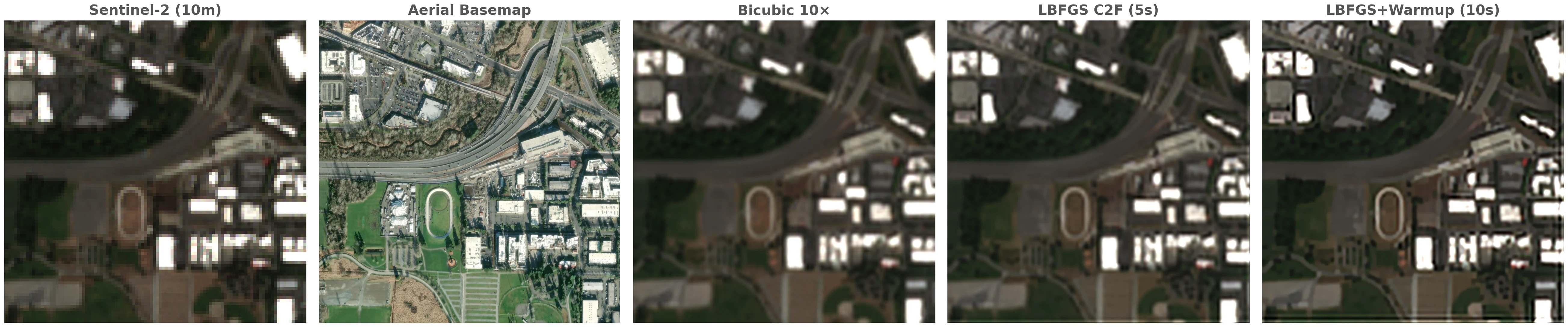
The bolded row was our sweet spot on this scene — the sharpest reconstruction without visible overfitting. At the final row’s settings the optimizer began fitting the noise as scene structure. “Mean LBFGS shift from init” is the mean adjustment away from the phase-correlation seed, not the absolute recovered shift.
The published S2 modulation transfer function suggests \(\sigma_{\text{psf}} \approx 3\)–4m for the 10m bands, which lands us in the bolded row of the table: in our reconstructions we saw meaningful sharpening down to roughly 8m features from 10m data, and visibly cleaner edges than bicubic upsampling. When we pushed \(\sigma_{\text{psf}}\) below 3m the optimizer began manufacturing structure the data doesn’t support – overfitting that looked plausible until we compared it against the aerial reference.
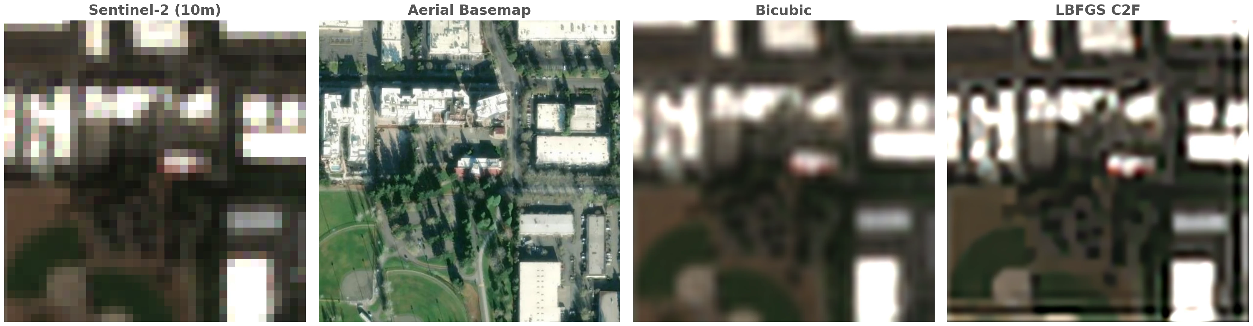
There is no neural network filling in plausible-looking texture. What you see is close to what the 32 observations support under the assumed forward model.
More observations reduce noise
Across our N-sweep, adding observations produced cleaner images but didn’t recover new spatial frequencies.
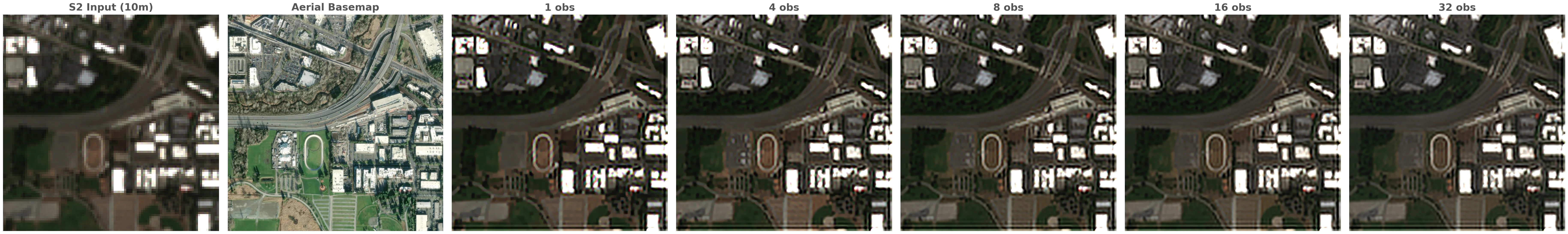
With the explicit sensor model, the fit stopped improving at about the same point whether we used 8, 16, or all 32 observations. More looks average down temporal variation from phenology, illumination, and atmosphere, but the 1.5m sub-pixel jitter is small relative to the 3 to 5m PSF — in this regime, multi-temporal fusion bought us SNR more than it bought us resolution.
Use a few well-chosen observations for sharper edges; add more only when you need denoising.
Fast in practice
The whole pipeline runs on a single GPU. At the 3 m default splat spacing, a 256 × 256 crop (~730k splats) fits in 30–150 seconds depending on configuration, and the full 987 × 1011 scene (~11M splats) fits in around 5 minutes. The biggest single speedup comes from handing the joint optimization to LBFGS after a brief Adam warmup:
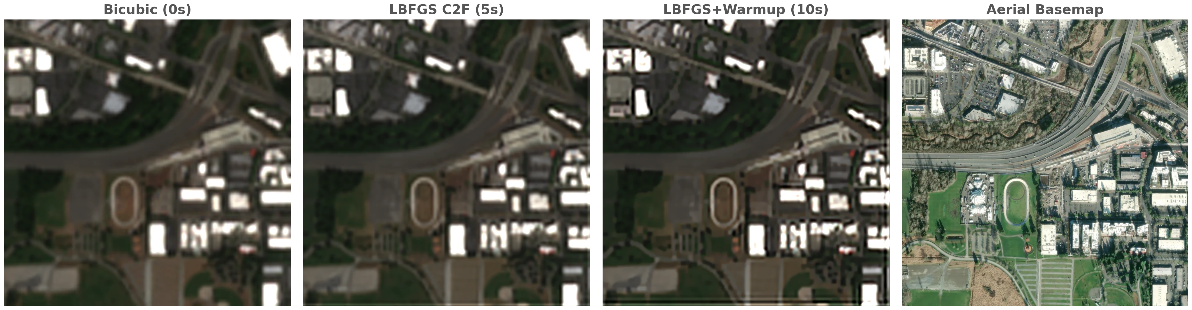
A few hundred Adam steps find a sane neighborhood – LBFGS’s quasi-Newton update can struggle with poor initialization – then LBFGS takes over. We found that with exact gradients through erf, LBFGS converged quickly and stably across the configurations we tried, and that the only knob that meaningfully changed outputs was \(\sigma_{\text{psf}}\). Varying the rest of the regularization (TV weight, splat spacing, \(\sigma_{\text{splat}}\)) had little visual impact in our experiments.
Conclusion
This formulation is a good fit when you want a per-scene, training-free reconstruction that runs end-to-end in minutes on a single GPU and handles multiple bands without extra cost. It is most useful when downstream users need to trust the pixels — change detection over time, visual inspection, or basemap production for areas without sub-meter coverage.
If you genuinely need sub-meter recovery from 10m data, you need something else. A learned prior trained on paired low- and high-resolution data (diffusion models, ESRGAN, and similar approaches), or an external structural reference like an aerial basemap or a sharper sensor (PlanetScope, SkySat). We have experimented with basemap-conditioned versions of this same optimizer and they look sharper, but the sharpness comes from the basemap, not the S2 stack.
The code is around 500 lines of PyTorch, with the analytic erf-based renderer on the bottom and a thin Adam-then-LBFGS loop on top.
Bibliography
[1] Irani, M. and Peleg, S. “Improving resolution by image registration.” CVGIP: Graphical Models and Image Processing, 1991.
[2] Razzak, M. T., Mateo-García, G., Lecuyer, G., Gómez-Chova, L., Gal, Y., and Kalaitzis, F. “Multi-Spectral Multi-Image Super-Resolution of Sentinel-2 with Radiometric Consistency Losses and Its Effect on Building Delineation.” ISPRS Journal of Photogrammetry and Remote Sensing, 2023.
[3] Aybar, C., et al. “A radiometrically and spatially consistent super-resolution framework for Sentinel-2.” Remote Sensing of Environment, 2026.
[4] Sirko, W., Asiedu Brempong, E., Marcos, J. T. C., Annkah, A., Korme, A., Hassen, M. A., Sapkota, K., Shekel, T., Diack, A., Nevo, S., Hickey, J., and Quinn, J. “High-Resolution Building and Road Detection from Sentinel-2.”, 2024.
Footnotes
Published Sentinel-2 modulation transfer function (MTF) numbers fold in both the optical blur and the 10m pixel integration. The forward model below handles the pixel integration explicitly (it integrates each splat over a 10m × 10m footprint via
erf), so the \(\sigma_{\text{psf}}\) in our equations is the residual optical and product blur on top of that, not the full system response.↩︎erfis the error function: \(\text{erf}(z) = \tfrac{2}{\sqrt{\pi}} \int_0^z e^{-t^2}\,dt\). Up to a linear rescaling, it gives the integral of a Gaussian over a half-line, which is exactly what we need to integrate a Gaussian over a finite pixel footprint.↩︎
Citation
@online{robinson2026,
  author = {Robinson, Caleb and Corley, Isaac},
  title = {Gaussian {Splat-based} {Satellite} {Image} {Super}
    {Resolution}},
  date = {2026-05-12},
  url = {https://geospatialml.com/posts/sentinel2-superresolution/},
  langid = {en}
}