ThroughputBench: How fast can a deep learning model map the Earth?
The abundance of open satellite imagery and advances in geospatial ML and remote sensing methods have made it possible to monitor a growing list of variables directly from orbit. Burke et al. (2021, Science), for example, reviewed how satellite imagery combined with machine learning can measure outcomes directly linked to the UN’s Sustainable Development Goals — population, economic livelihoods, infrastructure quality, land use, informal settlements, agricultural productivity, and others. Operational systems like Hansen’s global forest change product, and Google’s Dynamic World near-realtime land cover dataset are examples of planetary-scale monitoring with machine learning.
Modeling these variables well is one challenge. Scaling those models across the entire globe, on every new acquisition is a different challenge — and the choices you make at modeling time decide whether the second one is feasible at all. Take Dynamic World: Brown et al. report that they evaluate ~12,000 Sentinel-2 scenes per day and process about half after cloud filtering, so a new Dynamic World image lands roughly every 14.4 s — ~2 million Sentinel-2 tiles per year, or ~4 billion 224×224 patch-equivalents at 10 m. The paper itself notes the architecture they use to do this is “almost 100× smaller than U-Net or DeepLab v3+ baselines.”
An accurate model that is too expensive to run frequently at planetary scale may not be operationally useful. However, we couldn’t find anywhere this is benchmarked (although timm has a good benchmark script/results). So if you want to know whether ConvNeXt-B at fp16 on a V100 is cheaper than EfficientNet-B4 on an H100 for a global Sentinel-2 sweep, the answer today is to figure it out yourself.
Same imagery, same hardware, ~205× difference on the bill. Mapping the entire planet on every Sentinel-2 acquisition costs ~$30/year with MobileNetV3-S — or ~$6,150/year with ViT-L/8.
This post is about that gap! We built ThroughputBench — an extensible harness that measures model inference throughput for 33 common vision backbones plus 12 encoders across five geospatial foundation model families (DOFA, CROMA, SenPaMAE, Galileo, OlmoEarth), on whatever GPU you point it at, and serializes the results to a CSV. We’ve run the full matrix on two devices so far — raw results: V100, H100. You can see them summarized below, or play with our interactive viewer that shows how fast each model can sweep across Earth’s land surface.
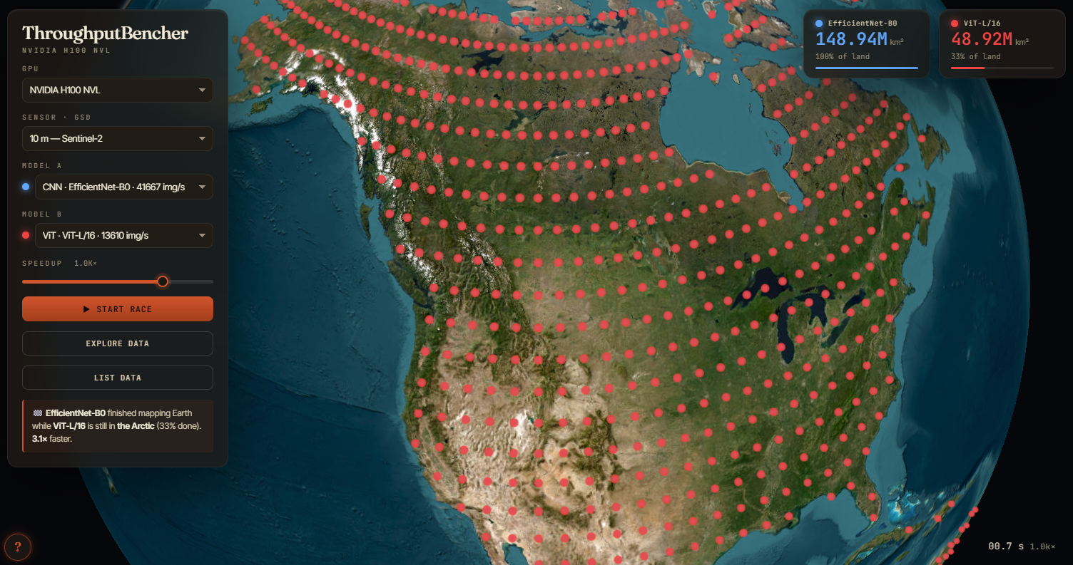
Figure 1: The interactive viewer — pick two models and a GPU, and see them race over Earth’s land surface!
Our results show that on a H100 GPU, the same ~4 B-patches/year Dynamic World workload takes:
- ~10 GPU-hours/year (~$30)1 with MobileNetV3-S throughput (115K img/s, fp16, compiled) — the cheapest backbone in the matrix.
- 21 GPU-hours/year (~$65) with ResNet-18 throughput (53K img/s, fp16, compiled)
- 430 GPU-hours/year (~$1,340) with ViT-L/16 throughput (2,585 img/s, bf16, compiled)
- ~970 GPU-hours/year (~$3,020) with the same ViT-L/16 with fp32 + no compile (1,147 img/s) — the precision and compile axes alone are ~2× on a single backbone.
- ~1,840 GPU-hours/year (~$5,720) with OlmoEarth-Large/8 throughput (604 img/s, bf16, compiled).
- ~1,980 GPU-hours/year (~$6,150) with ViT-L/8 throughput (562 img/s, bf16, compiled)2 — the most expensive backbone in the matrix, ~205× the cost of MobileNetV3-S.
Note — our results specifically bypass dataloader overhead, which can be significant, and only measure GPU time; see Dataloader overhead.
Methods
We ran every (model × precision × compile-mode × input-shape) combination on each GPU, recorded forward-pass latency, and divided by total wall-clock time to get images/sec. We fix batch size at 512 across the matrix.3 A few details about the protocol:
- We isolate the model from the dataloader. A pre-allocated batch sits on the GPU; we time only the model forward pass plus
cuda.synchronize(). Real pipelines have host→device transfer and disk I/O too, but we deliberately exclude both so what’s left is just the model and the precision (we revisit the dataloader cost in Dataloader overhead). - We warm up before timing. Twenty warmup iterations clear the
cudnnautotuner and any JIT compilation; then peak-memory stats reset and timing starts. Each cell runs for at least 30 seconds. Throughput is total images divided by total wall time, not the mean of per-iteration rates. - The GPU has to be idle. The benchmark harness checks for other processes on the GPU and aborts if it finds any.
- Encoder-only. Every model runs as the classification backbone alone, no segmentation decoder attached, so hierarchical CNNs and plain ViTs pay the same accounting.
- What “fp32” means depends on the GPU. On Ampere-and-newer GPUs (A100, H100), our
fp32rows are actually TF32 — 10-bit-mantissa Tensor Cores; on V100 they’re true IEEE-754 fp32. Atf32_enabledcolumn in the CSV disambiguates. (See the dtype primer below for what TF32 means.)
If you’re already comfortable with the difference between fp32, fp16, bf16, AMP, and TF32, skip this. Otherwise:
- fp32 (single-precision float) — 32 bits, what most PyTorch code uses by default. Slow on modern GPUs because it doesn’t run on Tensor Cores.
- TF32 — Ampere-and-newer NVIDIA GPUs run
fp32matmuls on Tensor Cores at TF32 precision (10-bit mantissa instead of 23-bit) when you settorch.set_float32_matmul_precision("high"). We enable this, so on H100 our “fp32” rows are TF32; on V100 (Volta) they’re true IEEE-754 (V100 has no fp32 Tensor Cores). - fp16 (half-precision) — 16 bits, runs on Tensor Cores at ~2× the throughput of TF32 (and ~8× of IEEE fp32 on V100). Numerical range is narrower; some models need loss scaling for training, but inference is usually fine.
- bf16 (brain float) — 16 bits with the same exponent range as fp32 but only 7 mantissa bits. Hardware-supported on Ampere+ (A100, H100); not supported on V100. More numerically stable than fp16 for some workloads.
- AMP (automatic mixed precision) — PyTorch’s
torch.autocastkeeps the model in fp32 and dynamically casts individual operations to fp16/bf16 per a built-in op list. Lower-overhead path to half: the wrapper code keeps running in fp32, only the heavy matmuls drop to half.
GPU-generation cheat sheet:
| Code name | Example cards | TF32 (fp32 Tensor Cores)? | bf16? |
|---|---|---|---|
| Volta | V100 | no | no |
| Ampere | A100, RTX A6000, RTX 30-series | yes | yes |
| Hopper | H100, H200 | yes | yes |
| Ada Lovelace | RTX 6000 Ada, L40 / L40S, RTX 40-series | yes | yes |
| Blackwell | B100, B200, GB200, RTX PRO 6000 Blackwell, RTX 50-series | yes | yes |
When this post says “Ampere+” or “modern GPUs” it means Ampere or newer (basically anything ≥ A100).
Models cover 33 architectures spanning five families — classical CNNs (ResNet, EfficientNet, ConvNeXt, MobileNetV3, RegNetY), plain ViTs (ViT, DeiT3, DinoV3), hierarchical ViTs (Swin, BEiT), and CNN-ViT hybrids (CoAtNet) — plus 12 encoders from five recent geospatial foundation model families4: DOFA (Xiong et al. 2024), CROMA (Fuller et al., NeurIPS 2023), SenPaMAE (Prexl & Schmitt, DAGM 2024), Galileo (Tseng et al., ICML 2025), and OlmoEarth (Herzog et al., CVPR 2026). Precisions are fp32, fp16, bf165, and amp. Compile modes are none and default (torch.compile with default Inductor settings).6
We benchmark each timm model across input sizes that match the geo-FMs we want to compare it against ({64, 120, 128, 144, 224}-pixel side, {2, 3, 10, 12} channels) so we can do shape-for-shape comparisons. We run each geo-FM at its pretraining shape: DOFA-{B,L}/16 at 3×224×224, CROMA-Optical at 12×120×120, CROMA-SAR at 2×120×120, SenPaMAE-B/16 at 3×144×144, Galileo-{Nano,Base,Large}/8 at 10×64×64, OlmoEarth-{Nano,Tiny,Base,Large}/8 at 12×128×128.7
Results
Mapping the Earth
A global scale Sentinel-2 monitoring job needs to process ~4 billion 224×224 patches/year (~12,000 tiles/day × half kept after cloud filter × ~1,950 patches/tile × 365 days). On an H100 GPU at each model’s best precision + compile, that costs anywhere from ten to ~2,000 GPU-hours — roughly $30 to $6,150/year at $3.11/hr per H100. This ~205× spread is what makes model choice an important lever for planetary scale jobs: the fastest backbone runs the entire job in tens of GPU-hours, while the heaviest one (ViT-L/8, the heaviest-compute vanilla ViT in our matrix) needs the equivalent of nearly three months of continuous H100 time.
Everything in this post is model-forward time only — a model-only lower bound for our specific stack (PyTorch eager + torch.compile, no TensorRT, ONNX export, quantization, CUDA graphs, or model surgery, all of which can move the floor further). Real deployment pipelines stack multipliers on top:
- Patch overlap — sliding-window inference typically overlaps adjacent patches to eliminate edge artifacts in the output. For example, a 50% overlap on both axes ⇒ ~4× more patches than the non-overlap count.
- Test-time augmentation — some pipelines ensemble each patch’s predictions across flips and rotations, typically 4×–8× more forward passes per patch.
- Dataloader overhead — we pre-allocate a batch on the GPU and time only the model (see Dataloader overhead below). Real pipelines spend 30–50% of wall time on host→device transfer and I/O.
These compose multiplicatively, so a realistic production setup can easily land 10–30× higher than the headlines above.
Browse the fp32 numbers
The table below shows our results for every model at fp32, compile_mode=none, on V100 and H100. Click a column header to sort, click a family chip to hide/show that family.
Note, the Input (C×HW) column is what each row is actually running. All timm models in this table run at 3×224 (standard ImageNet); the geo-FMs run at their pretraining shapes (12×120, 12×128, 10×64, 3×144, 2×120, 3×224 — so DOFA is the only geo-FM in the same shape as the timm rows). That means the img/s column is not directly comparable between rows with different shapes — Galileo-Nano/8 at 4,785 img/s is processing 64×64 patches, not 224×224 ones. The MPx/s column (channels × H × W × img/s, in megapixels per second) is the closest like-for-like throughput across shapes, though it still doesn’t account for the fact that the model is doing different amounts of work per pixel. The MACs (G) column counts multiply-accumulate operations in a single forward pass (in billions): one MAC is one multiply plus one accumulate, and FLOPs ≈ 2 × MACs. We use it as a rough compute budget for a model at a given input shape — bigger MACs means more arithmetic per image, though as we’ll see in the geo-FM section, MACs alone don’t predict throughput.
Sort by H100 img/s to see the throughput ladder; sort by MPx/s to compare across input shapes; click a family chip to focus on one architecture family.
Geo-FMs vs. matched-MAC vanilla baselines
The geo-FMs run at different input shapes with different numbers of input channels (12×128, 10×64, 12×120, 2×120, 3×144), so a head-to-head 3×224 comparison would be unfair to most of them. A fairer test: pair each geo-FM with the timm/DinoV3 model whose MAC count is closest, then compare throughput at fp32 + no compile so what’s left is just the architecture and the wrapper. For the smaller geo-FMs the closest-MAC comparator is naturally at the same input shape; for the largest ones (Galileo-Large/8, OlmoEarth-Large/8, OlmoEarth-Base/8) the only timm/DinoV3 models with comparable MAC budgets are the big ViTs at 3×224 — so we pair across shapes there, with the comparator’s shape noted in the table.
| Geo-FM | Native input | MACs (G) | Geo img/s | Closest-MAC comparator | shape | comparator img/s | Geo / comp |
|---|---|---|---|---|---|---|---|
| DOFA-B/16 | 3×224 | 34.0 | 3,260 | ViT-B/16 (33.7 G) | 3×224 | 3,315 | 0.98× |
| DOFA-L/16 | 3×224 | 119.7 | 1,126 | ViT-L/16 (119.3 G) | 3×224 | 1,147 | 0.98× |
| CROMA-Optical | 12×120 | 40.4 | 2,327 | Swin-L (35.2 G) | 12×120 | 2,294 | 1.01× |
| CROMA-SAR | 2×120 | 20.1 | 4,629 | ConvNeXt-L (17.2 G) | 2×120 | 5,199 | 0.89× |
| SenPaMAE-B/16 | 3×144 | 41.4 | 2,889 | Swin-L (41.2 G) | 3×144 | 1,881 | 1.54× |
| Galileo-Nano/8 | 10×64 | 0.5 | 4,785 | RegNetY-4GF (0.7 G) | 10×64 | 25,626 | 0.19× |
| Galileo-Base/8 | 10×64 | 54.4 | 1,349 | ConvNeXt-L (68.7 G) | 3×224 | 1,449 | 0.93× |
| Galileo-Large/8 | 10×64 | 302.1 | 393 | ViT-H/14 (323.8 G) | 3×224 | 440 | 0.89× |
| OlmoEarth-Nano/8 | 12×128 | 1.3 | 5,617 | ResNet-18 (1.4 G) | 12×128 | 44,355 | 0.13× |
| OlmoEarth-Tiny/8 | 12×128 | 8.2 | 2,752 | ResNet-152 (7.8 G) | 12×128 | 6,398 | 0.43× |
| OlmoEarth-Base/8 | 12×128 | 130.8 | 602 | ViT-L/16 (119.3 G) | 3×224 | 1,147 | 0.53× |
| OlmoEarth-Large/8 | 12×128 | 464.3 | 205 | ViT-L/8 (474.4 G) | 3×224 | 185 | 1.11× |
This splits the geo-FMs into two camps: ones whose input handling is essentially free, and ones whose input handling adds work that matters mostly at small model sizes.
DOFA, CROMA, and SenPaMAE are timm-class encoders with remote-sensing-aware inputs. DOFA-B/16 lands within 2% of ViT-B/16’s throughput at the same input shape; DOFA-L/16 within 2% of ViT-L/16. In this benchmark we don’t measure a meaningful overhead from the wavelength-conditioned dynamic patch embed. CROMA stays close to or above the closest-MAC timm backbone, and SenPaMAE outpaces Swin-L at matched MACs (1.54×) — it’s a plain ViT-B inside; we suspect Swin’s window attention contributes more small ops per FLOP, though we haven’t profiled to confirm. CROMA and DOFA trail their same-shape timm baselines mainly because they’re capped at fp32 + amp; SenPaMAE has full half-precision support and cashes it in (best H100 = 6,630 img/s at bf16 + compile, 2.3× the fp32 baseline).
Galileo and OlmoEarth tokenize each image as multiple bandsets — groups of spectral channels processed with separate patch embeddings. OlmoEarth at 12×128 with patch 8 produces 16×16 × 3 bandsets × 1 timestep = 768 tokens per image (vs. a vanilla ViT’s 256 at the same shape); Galileo at 10×64 with patch 8 produces 8×8 × 5 bandsets × 1 timestep = 320 tokens. On top of that, both wrappers run the multi-modal multi-timestep code path the models were trained for — per-timestep position embeddings still computed at T=1, modality-dispatch logic, and host-side reshaping (Galileo’s format_input, OlmoEarth’s MaskedOlmoEarthSample packing) — which adds several CPU ops to every forward.
How much this hurts throughput depends on size. At the small end, the picture is consistent with wrapper overhead dominating a tiny encoder: Galileo-Nano/8 trails an equivalent-MAC RegNetY by ~5×, and OlmoEarth-Nano/8 trails ResNet-18 by ~8×. At the large end, the encoder cost grows past whatever wrapper overhead exists and the geo-FMs catch up: Galileo-Large/8 runs at 0.89× of ViT-H/14 at matched MACs, and OlmoEarth-Large/8 actually runs faster than ViT-L/8 at matched MACs (205 vs 185 img/s, 1.11×) — once the encoder is big enough, the per-batch cost of the bandset and time-axis handling looks like a small share of total time.
A useful corollary: In this benchmark, MACs become more predictive of throughput at the largest scales, and less so at the small end. At 464 G MACs, OlmoEarth-Large/8 (205 img/s) and ViT-L/8 (185 img/s) land within 11% of each other on H100 fp32 + no compile — both appear to be compute-bound. At the small end the picture inverts: OlmoEarth-Nano/8 has 1.3 G MACs but runs at 13% of a same-MAC ResNet-18 (44,355 img/s). Without a profiler trace we can only speculate, but a plausible reading is that the ResNet’s 1.3 G is dominated by a few big matmuls that fuse into a handful of kernels, while the OlmoEarth wrapper’s many small per-modality / per-bandset ops launch hundreds of GPU kernels per batch. If a fixed per-batch wrapper cost is roughly constant across model sizes, then as the encoder grows, that cost takes up a smaller fraction of total time.
Cheaper isn’t automatically better. Large models exist because, in practice, they tend to deliver better downstream accuracy. The OlmoEarth paper (Herzog et al., CVPR 2026), for example, shows a clear monotonic increase in average task performance going from Nano → Tiny → Base on the benchmarks they evaluate — at the cost of the throughput we measure here. Throughput is only half the picture; the deployment question is which model is cheapest at your required accuracy — and accuracy is a question this post deliberately doesn’t answer. Treat the numbers here as one axis of a two-axis decision; the other axis lives in the foundation-model papers themselves.
Dataloader overhead
Inference throughput numbers are notoriously hard to compare across reports because the measurement protocol is rarely consistent. The most common confound is the input pipeline — how each batch gets to the GPU before the model runs.
To isolate the dataloader cost from any specific image decoder or augmentation stack, we wrote benchmark_dataloader_ipc.py: it runs ResNet-18 against a best-case Dataset that returns a cached random tensor for every __getitem__ — no image decoding, no augmentation, no disk I/O. What’s left in the pipeline is just batching, worker-to-main-process IPC, pinning, and the host→GPU copy. For each batch size and worker count, we measure three timings:
- compute — model forward through a pre-allocated GPU batch, plus
cuda.synchronize(). Upper bound, no dataloader involved. - fetch-only — one batch out of the DataLoader, no model. Pure pipeline cost.
- end-to-end — fetch-only + host→GPU copy + compute. The realistic path.
For a single 1024×3×224×224 batch on V100 with ResNet-18 at num_workers=8, those three paths cost:
| Path | What runs in it | Time |
|---|---|---|
| compute | model forward + cuda.synchronize() (batch already on GPU) |
~218 ms |
| fetch-only | DataLoader batch fetch (__getitem__s on workers + IPC + pin_memory) |
~222 ms |
| end-to-end | fetch-only + host→GPU copy + compute (overlapped) | ~275 ms |
The fetch-only path (~222 ms) costs about as much as a full ResNet-18 forward pass (~218 ms) — and a chunk of the total wall time even after overlap. If two benchmark reports use different num_workers, different pin_memory settings, different host/device topology, or different storage backends, their throughput numbers measure different things. Worse, these confounds tend to compress the spread between models — if every backbone is bottlenecked on host→device transfer, ResNet-18 and ViT-L/16 look closer than they really are.
Worker count
Compute time per batch is steady at ~218 ms regardless of worker count; only the fetch path varies. With num_workers=1 the worker becomes the bottleneck and end-to-end throughput collapses to ~1,800 img/s (2.6× slowdown vs. compute). Two workers already get most of the benefit; 4–8 workers settles into the steady-state ~3,700 img/s band. Past 8 workers the picture is noisier — most configurations land in the same ~3,500–3,800 range, but occasional contention spikes drop throughput by 10–15%, presumably from main-process scheduling overhead with many concurrent workers:
| Workers | End-to-end img/s | Slowdown |
|---|---|---|
| 1 | 1,795 | 2.60× |
| 2 | 3,597 | 1.30× |
| 4 | 3,753 | 1.25× |
| 8 | 3,727 | 1.26× |
| 12 | 3,301 | 1.42× |
| 16 | 3,196 | 1.47× |
| 24 | 3,671 | 1.28× |
(batch=1024, pin_memory=True, V100, ResNet-18, dummy cached-tensor dataset; full sweep in the results CSV.)
The practical takeaway: realistic ResNet-18 V100 throughput at bs=1024 is ~3,727 img/s, not the ~4,690 the model-only timer reports — about a 20% headroom. With a real dataset that does decoding and augmentation, the gap will widen further. The headline numbers in this post are model-only; multiply through accordingly when budgeting real workloads, and watch worker count especially if you’re sharing CPUs with other processes.
Appendix: precision, compile, and cross-GPU effects
The headline numbers in this post all use each model’s best precision + compile config. This appendix unpacks how that “best” gets there — which families gain the most from torch.compile and half precision, how the GPU type interacts with all of it, and how the geo-FMs respond to the same axes.
The speedup you get from going to half precision and turning on torch.compile is not uniform across model families — and the family-by-family pattern is different on V100 than on H100. The table below is the median speedup over the fp32 + no-compile baseline at 224×3, across all models in each family:
H100 NVL — speedup over fp32 + no-compile
Bolded entries mark each row’s best configuration.
| Family | fp32 + compile | fp16 + compile | bf16 + compile | amp + compile |
|---|---|---|---|---|
| ResNet | 1.86× | 3.40× | 3.15× | 3.21× |
| EfficientNet | 1.94× | 2.95× | 2.79× | 2.83× |
| MobileNet | 1.79× | 2.91× | 2.61× | 2.72× |
| RegNet | 1.66× | 2.56× | 2.48× | 2.44× |
| DeiT | 1.12× | 2.39× | 2.47× | 2.32× |
| ConvNeXt | 1.23× | 2.27× | 2.33× | 2.19× |
| Swin | 1.49× | 2.26× | 2.33× | 2.20× |
| ViT | 1.05× | 2.23× | 2.33× | 2.19× |
| DinoV3 | 1.19× | 2.13× | 2.33× | 2.13× |
| BEiT | 1.06× | 2.09× | 2.17× | 2.04× |
| CoAtNet | 1.21× | 1.71× | 1.71× | 1.69× |
V100 — speedup over fp32 + no-compile
| Family | fp32 + compile | fp16 + compile | amp + compile |
|---|---|---|---|
| DinoV3 | 0.99× | 5.05× | 4.94× |
| BEiT | 1.04× | 4.85× | 4.54× |
| ViT | 1.02× | 4.81× | 4.68× |
| DeiT | 1.04× | 4.37× | 4.23× |
| ConvNeXt | 1.08× | 4.29× | 4.11× |
| ResNet | 1.20× | 4.00× | 3.96× |
| Swin | 1.17× | 3.87× | 3.75× |
| CoAtNet | 1.21× | 3.60× | 3.57× |
| RegNet | 1.03× | 3.03× | 2.97× |
| EfficientNet | 1.46× | 2.99× | 2.97× |
| MobileNet | 1.42× | 2.66× | 2.60× |
We find:
Plain ViTs see a much bigger lift on V100 than on H100. BEiT-L/16 goes 5.05× faster on V100 with fp16 + compile, but only 2.07× on H100. ViT-B/16 sees 4.81× on V100, 2.23× on H100. The reason is that V100’s fp32 matmul path doesn’t use Tensor Cores at all — it runs on the regular CUDA cores at ~16 TFLOPs. fp16 unlocks Volta’s V100 Tensor Cores at ~125 TFLOPs (~8× peak ratio), and ViTs are mostly big matmuls — exactly the workload Tensor Cores were built for — so they cash in nearly the full speedup. On H100, the fp32 rows are already TF32 (Tensor Cores with a 10-bit mantissa), so fp16 only widens the lane that’s already open — ~2× peak ratio, not 8×. The V100 fp16 cliff for transformers is real, but it’s a measure of how bad V100 fp32 is, not how good V100 fp16 is.
CNNs are the opposite — bigger lift on H100, smaller on V100. ResNet sees 3.40× on H100 vs. 4.00× on V100; MobileNet sees 2.91× vs. 2.66×. CNNs spend a much larger fraction of their wall time on small, non-matmul ops (depthwise convs, BN, activations, kernel launches), so the compute speedup of half precision is diluted. On H100 the smaller-ops penalty is also smaller (faster scheduler, larger SMs), which is why MobileNetV3-S clears 115K img/s.
torch.compile alone (fp32 + compile) does very little. On both GPUs the median lift across families is in the 1.0–1.9× range. The big wins are paired: precision and compile. Compiled fp32 alone rarely justifies the build time.
CoAtNet is an outlier. Hybrid CNN-ViT, smallest precision lift on H100 (1.71×). We aren’t sure why (but reproduced this several times)!
GPU choice vs. model choice
Stack the precision/compile lift on top of the GPU change and you get the full cross-GPU picture. Fix the model, take each GPU’s best precision + compile config: ResNet-18 throughput goes 14,762 → 53,478 img/s (V100 → H100, 3.6×); ViT-L/16 goes 529 → 2,585 (4.9×); Galileo-Large/8 goes 183 → 843 (4.6×). At the 4 B-patches/year baseline, that translates to 75 → 21 GPU-h/yr for ResNet-18, 2,100 → 430 for ViT-L/16, and ~6,070 → ~1,320 for Galileo-Large/8.
Once AMP is unlocked across the matrix on V100 (and SenPaMAE/OlmoEarth gain full fp16/bf16), the cross-GPU spread is roughly flat at 3–5× across families — the geo-FMs aren’t the outliers they were when V100 was stuck on the slowest fp32 path. The point worth keeping: the spread across models on a single GPU (~205× from MobileNetV3-S to ViT-L/8) dwarfs the spread across GPUs for any single model (3–5×). Model choice dominates GPU choice for this workload.
Links
- Code: github.com/calebrob6/throughput-bench
- Interactive viewer: calebrob.com/throughput-bench
- Results CSVs:
results/(V100, H100 NVL)
Footnotes
Costs throughout this post use $3.11/hr per H100 NVL, the average across cloud providers from getdeploying.com/gpus/nvidia-h100. Costs scale linearly with GPU-hours, so swap in your own rate if you’ve negotiated a better one.↩︎
ViT-L/8 is non-standard — vanilla ViT-L is typically
/16. We added it (along with ViT-H/14, ViT-G/14, and DinoV3-H+/16) as same-compute / same-token-count comparators for the larger geo-FMs. At 3×224 with patch size 8, ViT-L/8 produces (224/8)² = 784 tokens, roughly matching OlmoEarth-Large/8’s 768 tokens at 12×128, and at 474 G multiply-accumulates per forward pass (MACs) vs OlmoEarth-Large/8’s 464 G it’s a near-MAC match. We use it as the apples-to-apples vanilla ViT for the large geo-FMs in the Geo-FMs vs. shape-matched timm baselines section.↩︎The only models that didn’t fit at 512 were CoAtNet-0 and CoAtNet-2, both of which the harness halved to 256 on both V100 and H100. Every other model fits at 512 on both GPUs.↩︎
Galileo and OlmoEarth are time-series multimodal models that can ingest a sequence of images across multiple modalities; we benchmark them in their simplest configuration (single image, single timestep, Sentinel-2 only). Both wrappers use
max_patch_size=8andmax_sequence_length=1. Both also tokenize each image as multiple bandsets (groups of spectral channels with separate patch embeddings): OlmoEarth at 12×128 produces 16×16 × 3 bandsets × 1 timestep = 768 tokens per image (12-band L2A); Galileo at 10×64 produces 8×8 × 5 bandsets × 1 timestep = 320 tokens (10-band S2 split into RGB / Red Edge / NIR-10m / NIR-20m / SWIR). DOFA, CROMA, and SenPaMAE are not time-series models, so their wrapper settings are minimal: DOFA passes the per-channel wavelength tensor (Sentinel-2 wavelengths truncated tonum_channels); CROMA dispatches by modality ("optical"→ 12-band Sentinel-2,"SAR"→ 2-band Sentinel-1); SenPaMAE uses dummy SRF and GSD constants (the forward needs them but they don’t affect throughput). All five families run with random weights, since throughput doesn’t depend on the parameter values. Full wrapper code:geo_models.py.↩︎We skip bf16 on V100 — Volta has no hardware support for it (Ampere added it).↩︎
The harness also exposes
max-autotune, but we didn’t include it in this sweep.↩︎The Galileo paper (Tseng et al. 2025, Table 12) only releases Nano, Tiny, and Base checkpoints. Galileo-Large/8 in our matrix is a synthetic ViT-Large (1280 dim × 24 depth × 16 heads, 474.7M params) plugged into the same wrapper — a “what does this architecture look like at ViT-Large scale” data point, not an officially released model.↩︎
Citation
@online{robinson2026,
  author = {Robinson, Caleb and Corley, Isaac},
  title = {ThroughputBench: {How} Fast Can a Deep Learning Model Map the
    {Earth?}},
  date = {2026-05-04},
  url = {https://geospatialml.com/posts/throughput-bench/},
  langid = {en}
}